Different results of CMR algorithms in R – Part 3
This is the third part of my attempt to understand why two implementations of coupled monotonic regression (CMR) gave different answers. In Part 1, I compared the simple algorithm in pirst with the Java implementation in stacmr. In Part 2, I tried to make that comparison fair by supplying the Java solver with the partial order that is built into the simple algorithm.
The call in Part 2 looked right:
pirst:::easy_jCMRx(
  d$X,
  d$Y,
  partial = list(1:4, 5:8)
)
Nevertheless, the output now provides a clue that the partial order did not actually reach the solver. Retracing that calculation also answers the more basic question I should have asked first: what happens when I compare the algorithms using the squared-error criterion that they optimize?
Returning to the same example
I use the same simulated data and seed as in Part 2.
Instead of relying on the convenience wrapper, I now construct the input for jCMRx() explicitly. This makes it possible to fit the model once without constraints and once with the two within-condition chains.
The two vectors in partial say that rows 1 to 4 form one ordered chain and rows 5 to 8 form another. This is appropriate here because pirstsim() returns the four trace levels of condition 1 followed by the four trace levels of condition 2.
Repeating the comparison with squared deviations
easy_cmr() returns its rows in the fitted common order, so I merge its output with the observations using the experimental identifiers. The Java result retains the input order.
keys <- c("Condition", "Trace", "Measurement", "Person")
d_easy <- merge(d, fit_easy, by = keys)

residual_easy <- (
  as.matrix(d_easy[c("X.x", "Y.x")]) -
  as.matrix(d_easy[c("X.y", "Y.y")])
)
residual_java_free <- (
  as.matrix(d[c("X", "Y")]) - fit_java_free$x
)
residual_java_partial <- (
  as.matrix(d[c("X", "Y")]) - fit_java_partial$x
)

scores <- function(residuals) {
  c(
    absolute_error = sum(abs(residuals)),
    squared_error = sum(residuals^2)
  )
}

comparison <- rbind(
  "easy_cmr, partial order" = scores(residual_easy),
  "jCMRx, no partial order" = scores(residual_java_free),
  "jCMRx, partial order" = scores(residual_java_partial)
)

knitr::kable(comparison, digits = 8)| absolute_error | squared_error | |
|---|---|---|
| easy_cmr, partial order | 0.4945134 | 0.04878204 |
| jCMRx, no partial order | 0.5128164 | 0.03996091 |
| jCMRx, partial order | 0.4905439 | 0.04861529 |
This table resolves two questions at once.
First, the value printed for jCMRx in Part 2 was 0.5128164. That is exactly the absolute error of the unconstrained Java fit. The call in the post supplied partial to easy_jCMRx(), but the numerical result shows that the installed wrapper used for that execution did not pass it on as E to jCMRx().
The source file in my working copy now contains the forwarding call jCMRx(d, E = partial). The most likely explanation is that I changed the package source but rendered the post with an older installed namespace. Using pirst::: calls the installed package; editing R/cmr.R does not update that installation automatically. I cannot reconstruct the transient installed function after the fact, but the exact reproduction of 0.5128164 makes clear which model produced the old result.
Second, replacing absolute deviations with squared deviations reverses the ranking of the two fits that were actually compared in Part 2: the unconstrained Java fit has smaller squared error than easy_cmr(). But that comparison is not meaningful, because the Java solver was allowed to ignore the two within-condition orders. The fair comparison is between the first and third rows. With the same partial order, jCMRx() is slightly better under squared error. In fact, in this example it is also slightly better under absolute error.
A state-trace example: absolute versus squared error
Although the loss function was not the source of the constrained discrepancy here, absolute and squared error can certainly produce different monotone fits. Consider one condition measured at five ordered trace levels. All observed X and Y values are distinct. Variable Y increases with the trace, but X turns backwards over the three middle levels.
toy_sta <- data.frame(
  X = c(0.1, 0.9, 0.7, 0.2, 1.0),
  Y = c(0.1, 0.3, 0.5, 0.7, 0.9),
  Condition = 1,
  Trace = 1:5
)

pooled <- 2:4
absolute_level <- median(toy_sta$X[pooled])
squared_level <- mean(toy_sta$X[pooled])

fit_absolute <- toy_sta
fit_squared <- toy_sta
fit_absolute$X[pooled] <- absolute_level
fit_squared$X[pooled] <- squared_level

plot(
  toy_sta$X,
  toy_sta$Y,
  xlim = c(0, 1.05),
  ylim = c(0.05, 1.25),
  xlab = "Variable X",
  ylab = "Variable Y",
  main = "Two monotone fits to the same state-trace data",
  pch = 19
)
lines(toy_sta$X, toy_sta$Y, col = "grey60", lty = 3)
points(toy_sta$X, toy_sta$Y, pch = 19)
text(
  toy_sta$X,
  toy_sta$Y,
  labels = paste0("T", toy_sta$Trace),
  pos = c(3, 3, 3, 3, 1)
)

lines(fit_absolute$X, fit_absolute$Y, col = "steelblue", lwd = 2)
points(fit_absolute$X, fit_absolute$Y, col = "steelblue", pch = 1)

lines(fit_squared$X, fit_squared$Y, col = "firebrick", lwd = 2, lty = 2)
points(fit_squared$X, fit_squared$Y, col = "firebrick", pch = 2)

legend(
  "topright",
  legend = c("observed trace order", "minimum absolute error", "minimum squared error"),
  col = c("grey40", "steelblue", "firebrick"),
  pch = c(19, 1, 2),
  lty = c(3, 1, 2),
  lwd = c(1, 2, 2)
)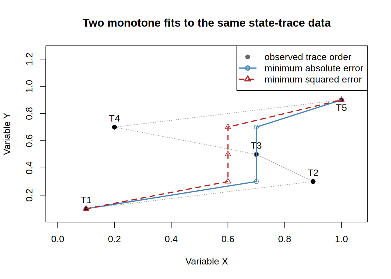
The observed path runs backwards in X from T2 through T4. Enforcing a nondecreasing state trace therefore pools those three X values into a common fitted level, while T1 and T5 remain unchanged. Ties in the fitted values are a normal consequence of isotonic regression even though none of the observed coordinates are tied. Minimizing absolute error puts the pooled level at the median of 0.9, 0.7, and 0.2, which is 0.7. Minimizing squared error puts it at their mean, which is 0.6.
toy_scores <- data.frame(
  criterion = c("absolute error", "squared error"),
  fitted_X = c(absolute_level, squared_level),
  absolute_error = c(
    sum(abs(toy_sta$X - fit_absolute$X)),
    sum(abs(toy_sta$X - fit_squared$X))
  ),
  squared_error = c(
    sum((toy_sta$X - fit_absolute$X)^2),
    sum((toy_sta$X - fit_squared$X)^2)
  )
)

knitr::kable(toy_scores, digits = 2, row.names = FALSE)| criterion | fitted_X | absolute_error | squared_error |
|---|---|---|---|
| absolute error | 0 | 3 | 9 |
| squared error | 1 | 4 | 6 |
For the pooled block, the absolute-error solution produces residuals 0.2, 0, and -0.5. The squared-error solution spreads the adjustment more evenly, producing residuals 0.3, 0.1, and -0.4. Its total absolute error is therefore larger, 0.8 instead of 0.7, but its squared error is smaller, 0.26 instead of 0.29. Squaring penalizes the largest residual more strongly and shifts the plateau away from the median towards the mean.
Thus, the same state-trace data and the same monotonicity constraint can lead to different fitted curves solely because the criterion changes. Both easy_cmr() and jCMRx() use squared error internally, however. The absolute-error calculation in Part 2 was a descriptive comparison, not the objective optimized by either method.
Why the constrained fits still differ
After applying the same partial order, the remaining squared-error difference is small:
\[ 0.04878204 - 0.04861529 = 0.00016675. \]
It is not just numerical rounding. The two functions reach their solutions differently.
At a high level, easy_cmr() builds the common order sequentially. It makes the best available insertion at each step, but it does not jointly reconsider all earlier choices. jCMRx(), by contrast, solves the joint constrained problem supplied through E. It can therefore attain a slightly smaller overall squared error.
What I learned from the comparison
The partial order written in the Part 2 call was the right one. The problem was that the result saved with that post came from the unconstrained Java model, showing that the wrapper used during rendering had not forwarded the argument to the underlying solver.
Once I bypass the wrapper and call jCMRx(..., E = partial) directly, the puzzle becomes much less mysterious. easy_cmr() and jCMRx() produce very similar constrained fits. The Java solution has a small but genuine advantage because it performs the joint optimization, whereas the simpler R implementation makes greedy insertion decisions.
The practical lesson is to inspect the objective as well as the fitted curve, and—especially when working on a package—to verify the function in the loaded namespace rather than assuming that an edited source file is already installed.
Outlook: opening the two black boxes
The next step is to explain how the two functions arrive at their answers. I want to follow this eight-point example through easy_cmr() one operation at a time: the initial within-condition isotonic fits, the candidate insertion positions, the squared error at each position, and the final common order. I will then trace how jCMRx() represents the same partial order through E and how it obtains the joint solution. That should reveal the precise decision at which the greedy path loses the small amount of squared error seen above.
pirst did not initially import stacmr; that dependency was added later while I was investigating the Java solver. Given that it is now available, the most direct route to an exact CMR null-model fit is to reuse jCMRx(). What pirst needs for this route is a reliable adapter that constructs the means, weights, and partial-order constraints, forwards them to jCMRx(), and returns fitted values in an unambiguous row order. The simpler easy_cmr() can remain useful for understanding and testing the procedure, but it does not have to carry the burden of being the exact optimizer.
Reusing jCMRx() need not be the final implementation choice. Speed is crucial for PIRST, especially once analyses involve many participants, permutations, and bootstrap samples. A native C++ implementation of the exact optimizer may therefore be worthwhile: it could be faster than the Java implementation, and Rcpp makes it easy to integrate C++ code into an R package. Before attempting that, I first need to understand and document both existing algorithms precisely. jCMRx() can then serve as the reference implementation against which a C++ version is tested for identical constraints, fitted values, and objective values, followed by benchmarks to determine whether a rewrite provides a meaningful speed advantage.