mimosa 0.6.1: Better Model Tables, Binary Outcomes, and Reproducible R Code
I have released mimosa 0.6.1, a substantial update to my graphical interface for two-level mixed models (Titz 2020).
mimosa has always had two use cases. It offers researchers a simple interface for clustered or repeated-measures 2-level data, but it was also designed for teaching. Students need only a browser: there is no complicated R installation, no package setup, and no development environment to configure before they can explore a mixed model.
Now that AI can perform much of an analysis for you, I see mimosa’s purpose as purely educational: helping students understand what a two-level model contains, how modeling choices change the result, and how the quantities in the output are calculated. This change in emphasis motivated several features in this release, especially the more transparent model table, the explanatory tooltips, and the generated R code.
Version 0.6.0 was the large feature release. Version 0.6.1 followed immediately with a small but important correction to downloaded tables, so 0.6.1 is the version to use.
A more informative model table
For teaching, this is the most important change. Mixed models are difficult partly because their variance components, correlations, ICC, and different R-squared measures are often presented as finished numbers without showing how they relate to one another. The new output makes this structure more explicit. In addition to the coefficient table, mimosa displays:
- the empirical fixed-effect variance,
- the random-effect variance components,
- the residual variance,
- the intraclass correlation coefficient (ICC), and
- marginal and conditional R-squared.
Random-slope variances and correlations are placed next to their corresponding predictor rather than being detached from the term they describe. This makes larger random-effects structures considerably easier to read.
The summary values also have detailed hover explanations. Hovering over an R-squared or ICC value shows both its interpretation and the variance components used in the calculation. The formulas are no longer hidden behind a single unexplained number.
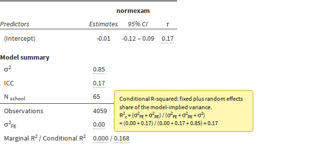
I wanted to be particularly careful here because there are several ways to calculate variance summaries for mixed models. Automated tests fit the same models used in published worked examples by Nakagawa and Schielzeth (2013) and Johnson (2014), then compare mimosa’s results with the published values. If a future code change alters one of those calculations unexpectedly, the test fails. The Johnson two-level Orange example can also be selected directly inside mimosa.
Dichotomous outcomes
Until now, mimosa was essentially a Gaussian mixed-model application. Version 0.6 adds automatic support for dichotomous dependent variables.
When the selected response has exactly two observed values, mimosa fits a generalized linear mixed model using lme4::glmer(..., family = binomial()) (Bates et al. 2015). Numeric outcomes with more than two values continue to use lme4::lmer(). Two-level factors, character variables, logical variables, and numeric variables can all be used as dichotomous responses.
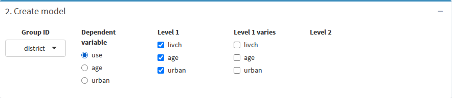
use variable and prepares a two-level model.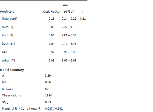
From a convenient interface back to reproducible R
A graphical interface is useful for constructing an analysis, but the result should not be trapped inside the interface. The new R analysis code panel therefore generates a complete, copyable script for the current model.
The script includes:
- reproducible data loading,
- the exact
lmer()orglmer()call, - any required conversion of a two-category response, and
- the
sjPlot::tab_model(model)call used to create the table.
Variable names that are not syntactically valid R names are quoted safely, and long formulas are wrapped so the code remains readable. A copy button places the complete script on the clipboard.
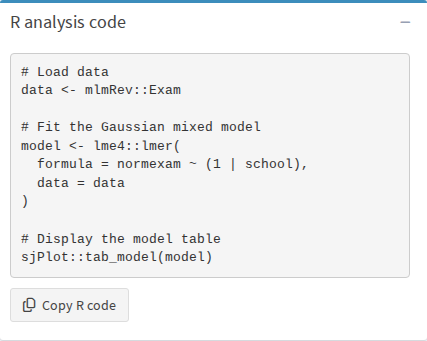
For teaching, this connects the graphical choices to the R code behind them. Students can construct a model visually, inspect the corresponding formula and function call, and then run or modify the generated script themselves. The interface is therefore not a dead end; it can be a bridge toward working directly in R.
Better guidance when data are imperfect
Real data rarely arrive in the tidy shape used in demonstrations. Version 0.6 improves several failure paths that previously produced vague messages or silent failures.
Grouping-variable detection now explains its reasoning, uses more robust repeated-measure thresholds, and warns when a proposed grouping variable has too many groups without repetition. The underlying diagnostics can be inspected outside the application with the exported explain_find_id() function.
Uploaded-file handling and character-encoding fallbacks are more robust as well. Singular fits, model-fitting errors, and cases with too few repeated groups now produce useful guidance instead of leaving an empty output region.
There are also smaller interface changes: additional two-level example data sets, a visible installed-version number, a reorganized output area, and consistent busy indicators for the model, R-code, and save-output panels.
A browser-only version with webR
There are now two hosted versions of mimosa. The regular mimosa.icu deployment still uses ShinyProxy and runs an ordinary R process on the server for each session. In addition, anyone can open the webR version directly from GitHub Pages. That version downloads a WebAssembly build of R and performs the analysis locally inside the browser.
The webR version requires no local R installation and no account, which makes it particularly attractive for teaching. I do, however, want to be honest about its current performance. It remains noticeably slower to start than a warm ShinyProxy session. Every page load creates a new in-browser R session and mounts the required WebAssembly packages, even when the files themselves are cached.
I reduced the exported dependency set from 154 to 52 entries and the generated site from roughly 217 MB to 125 MB. On a typical desktop, the interface now becomes usable after about 20 seconds, and the initial model table is usually ready after 30–40 seconds. Device and network speed still matter. The regular ShinyProxy deployment is therefore the better default for a lesson in which students should begin at the same time. The GitHub-hosted webR version is useful when a large group wants to use mimosa and the startup delay is acceptable. ShinyProxy naturally has a limit on simultaneous sessions, although the current capacity should be sufficient for typical class sizes.
Less glamorous, but important work
Much of this release is invisible. The automated suite now contains 279 test expectations and reaches 97.7% line coverage. It exercises Gaussian and binomial models, generated R code, uploads, downloads, reactive errors, and output diagnostics. GitHub Actions runs R package checks on Linux, Windows, and macOS and produces coverage reports.
The Docker image was also rebuilt around the current checkout. Dependency installation is cached separately from application code, development files are excluded from the build context, compiled libraries are stripped, and the application runs as a non-root user. Unused or unnecessarily heavy dependencies were removed where possible.
Why 0.6.1 followed so quickly
The new hover explanations exposed a small problem in 0.6.0: the downloaded standalone HTML table contained the tooltip bodies. Inside the application those explanations are hidden until the user hovers over a value, but the downloaded file does not include the app’s tooltip styling and could display them as ordinary table content.
Version 0.6.1 removes the interactive tooltip markup and explanatory text from the downloaded copy while preserving all visible estimates and summary values. The live table retains its tooltips. An automated test now checks this distinction whenever the package is tested.
Trying mimosa
The regular ShinyProxy application is available at mimosa.icu. The browser-only webR build is served directly from GitHub Pages and follows the development version on the master branch, so it may already contain changes made after the latest release. Its header marks the build as dev and shows the short commit hash of the exact version currently running.
To install the exact release from GitHub:
install.packages("remotes")
remotes::install_github("johannes-titz/[email protected]")
mimosa::run_app()
The source code, full change log, and issue tracker are in the mimosa GitHub repository. mimosa remains intentionally limited to two-level models. If your data require three or more levels or a substantially more complex model, a more general modeling interface—or direct R code—is the better tool.
If you try the new release and something behaves unexpectedly, please open an issue. With a relatively small project, reports from actual analyses and teaching sessions are especially valuable: they reveal combinations of data structures and modeling choices that even a fairly extensive automated test suite will not anticipate.