Different results of CMR algorithms in R – Part 2

After a fruitful meeting with Lukas, here is another attempt to understand the CMR-algorithms. Lukas explained to me that his easy_cmr algo always fits a partial order first for the two conditions. This is because the trace variable should cause a monotonic increase in both conditions, which totally makes sense if you are familiar with the paper by Prince, Brown, and Heathcote (2012).

Let’s go through the same steps, but now specificy the partial order for both conditions. This will allow us to see if jCMRx from stacmr will indeed produce a better fit with this partial order than the fit without any order.

librarian::shelf(monotonicity/stacmr, johannes-titz/pirst)

Consider the following case:

set.seed(1)
d <- pirstsim(cases = 1, nmeasures = 1, noise = .2)
st_plot(d)

res1 <- pirst:::easy_cmr(d)
points(res1$X, res1$Y, col = "steelblue", type = "b", pch = 22, lty = 2)

res2 <- pirst:::easy_jCMRx(d$X, d$Y, partial = list(1:4, 5:8))
res2_sorted <- res2[order(res2[, 2]), ]
points(res2_sorted[, 1], res2_sorted[, 2], col = "firebrick", type = "b",
       pch = 23, lty = 2)

legend(
  "bottomright",
  legend = c("easy_cmr", "jCMRx"),
  col     = c("steelblue", "firebrick"),
  pch     = c(22, 23),
  lty     = 1,
  pt.bg   = c("steelblue", "firebrick")
)

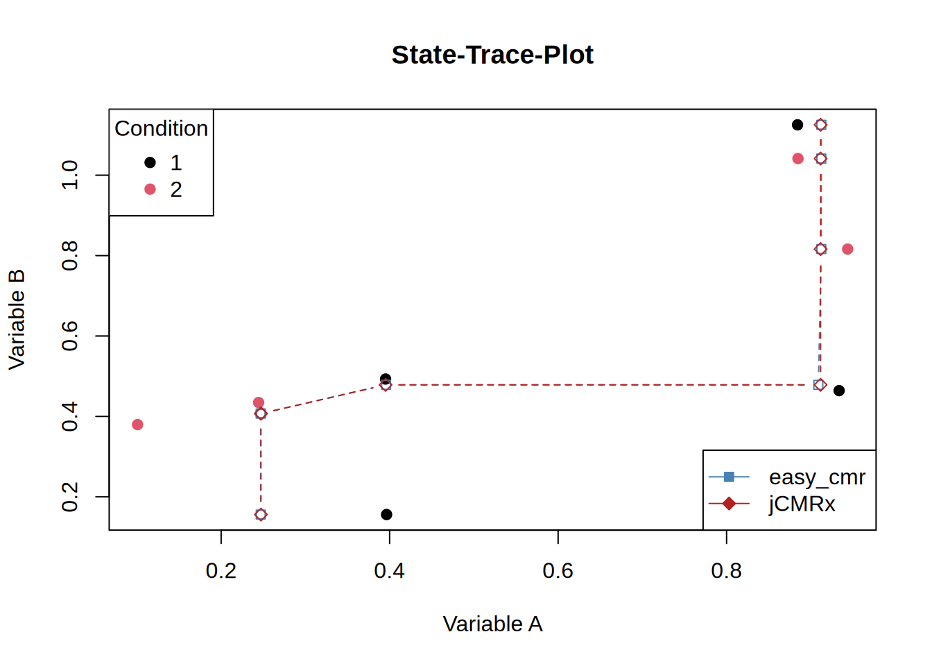
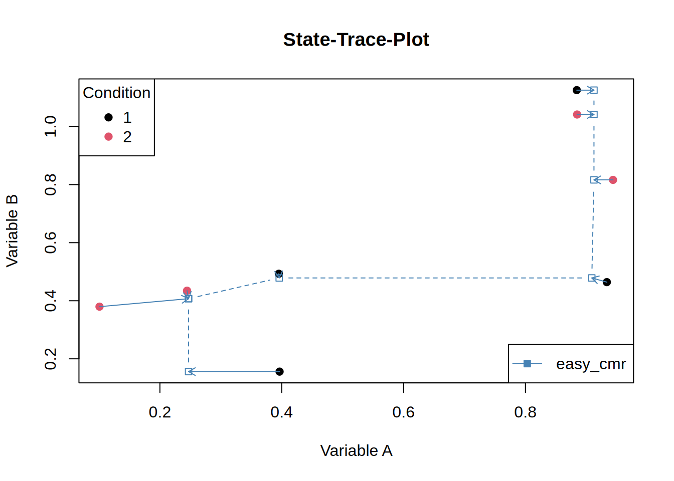
The two solutions clearly differ substantially, but which one is closer to the empirical data?

d_m <- merge(d, res1, by = c("Condition", "Trace", "Measurement", "Person"))
sum(abs(d_m[, c("X.x", "Y.x")] - d_m[, c("X.y", "Y.y")]))

[1] 0.4945134

sum(abs(d[, 1:2] - res2))

[1] 0.5128164

Indeed, Lukas’s algorithm yields the slightly better fit. However, this discrepancy might simply stem from how I am invoking the Java functions. I still need to determine whether the parameters model and E (the partial order) influence the results in unintended ways when they are omitted. Although the discrepancy is small, this is obviously not due to rounding errors.

Let’s add some arrows to see which points move:

st_plot(d)
points(res1$X, res1$Y, col = "steelblue", type = "b", pch = 22,
       lty = 2)
arrows(x0 = d_m$X.x, y0 = d_m$Y.x, x1 = d_m$X.y, y1 = d_m$Y.y, col = "steelblue",
       length = 0.08)

legend(
  "bottomright",
  legend = c("easy_cmr"),
  col     = c("steelblue"),
  pch     = c(22),
  lty     = 1,
  pt.bg   = c("steelblue")
)

st_plot(d)
points(res2[order(res2[, 1]), 1], res2[order(res2[,1]), 2], col = "firebrick",
       type = "b", pch = 23, lty = 2)
arrows(x0 = d$X, y0 = d$Y, x1 = res2[, 1], y1 = res2[, 2], col = "firebrick",
       length = 0.08)

legend(
  "bottomright",
  legend = c("jCMRx"),
  col     = c("firebrick"),
  pch     = c(23),
  lty     = 1,
  pt.bg   = c("firebrick")
)

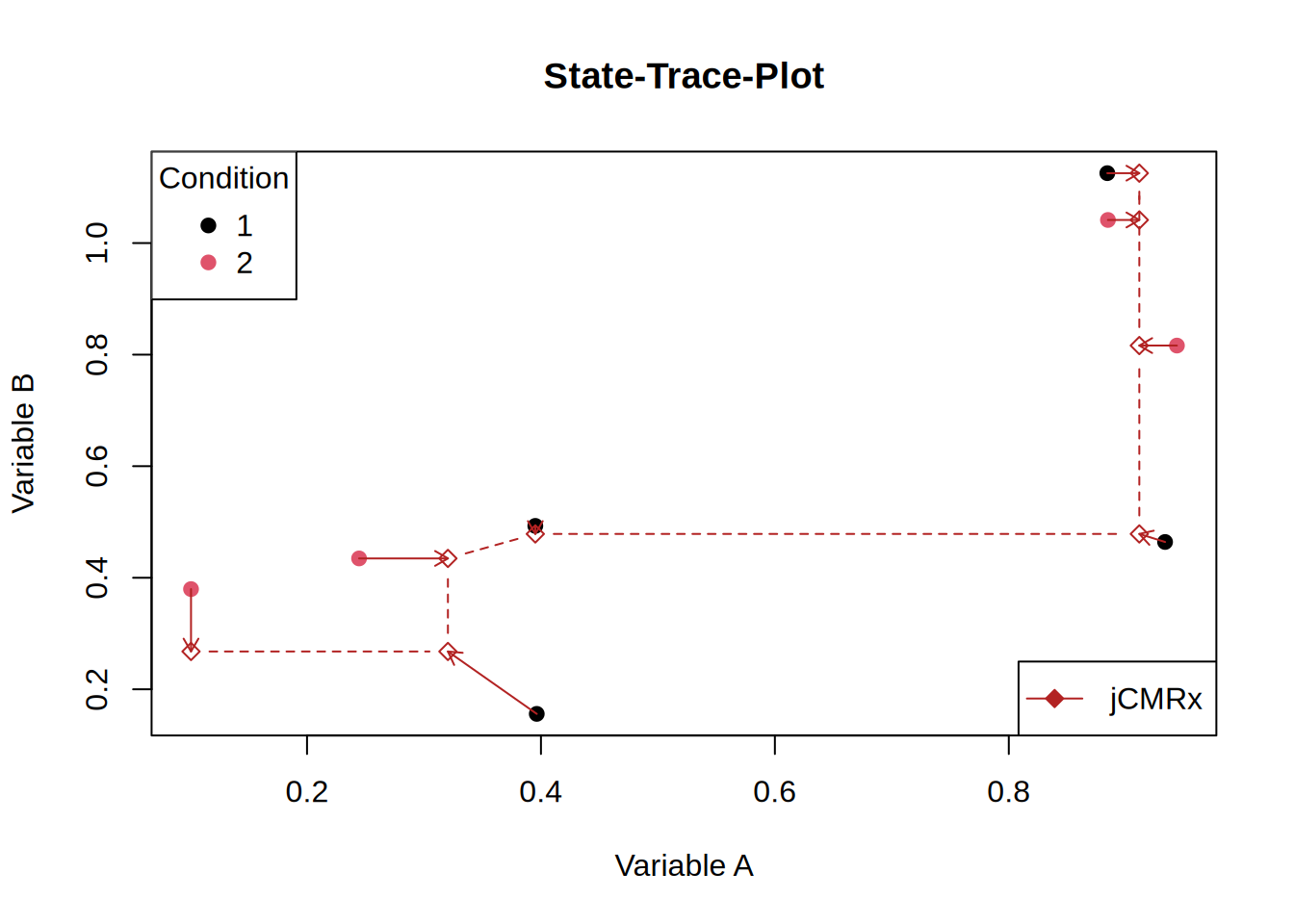
One rather puzzling aspect is that, for jCMRx, the last four points share the same abscissa value, whereas for easy_cmr only the final three points coincide on the abscissa, with the fourth-to-last point shifted slightly further to the left. I am not entirely certain whether this behaviour is expected and whether it is of any substantive relevance.

It is difficult to find an empirical data set that allows for a proper comparison—specifically one that uses the stacmr functions and for which published results are available. In the book by Dunn and Kalish (2018), only a single data set is suitable for a straightforward CMR comparison: the face-inversion data described from page 74 onwards. But even for this data set an algorithm that takes into account the partial order is required.

References

Dunn, John C., and Michael L. Kalish. 2018. State-Trace Analysis. Computational Approaches to Cognition and Perception. Cham: Springer International Publishing. https://doi.org/10.1007/978-3-319-73129-2.
Prince, Melissa, Scott Brown, and Andrew Heathcote. 2012. “The Design and Analysis of State-Trace Experiments.” Psychological Methods 17 (1): 78–99. https://doi.org/10/ff8czx.