Different results of CMR algorithms in R

Recently I wrote about the CMR algorithm (https://johannestitz.com/post/2025-11-25-sta-cmr/). Today, after running additional tests, I discovered discrepancies between the results produced by Lukas’s CMR implementation and those generated by the algorithms in stacmr and the corresponding Java library.

Before we begin, we install the required libraries (using librarian for convenience):

librarian::shelf(monotonicity/stacmr, johannes-titz/pirst)

Consider the following case:

set.seed(1)
d <- pirstsim(cases = 1, nmeasures = 1, noise = .2)
st_plot(d)

res1 <- pirst:::easy_cmr(d)
points(res1$X, res1$Y, col = "steelblue", type = "b", pch = 22, lty = 2)

res2 <- pirst:::easy_jCMRx(d$X, d$Y)
res2_sorted <- res2[order(res2[, 2]), ]
points(res2_sorted[, 1], res2_sorted[, 2], col = "firebrick", type = "b",
       pch = 23, lty = 2)

legend(
  "bottomright",
  legend = c("easy_cmr", "jCMRx"),
  col     = c("steelblue", "firebrick"),
  pch     = c(22, 23),
  lty     = 1,
  pt.bg   = c("steelblue", "firebrick")
)

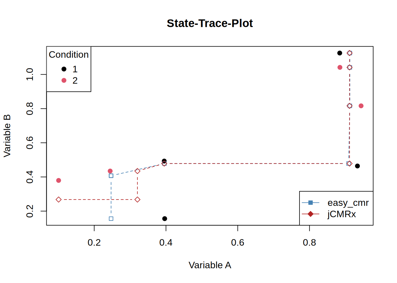
The two solutions clearly differ substantially, but which one is closer to the empirical data?

d_m <- merge(d, res1, by = c("Condition", "Trace", "Measurement", "Person"))
sum(abs(d_m[, c("X.x", "Y.x")] - d_m[, c("X.y", "Y.y")]))

[1] 0.4945134

sum(abs(d[, 1:2] - res2))

[1] 0.5128164

Indeed, Lukas’s algorithm yields the slightly better fit. However, this discrepancy might simply stem from how I am invoking the Java functions. I still need to determine whether the parameters model and E (the partial order) influence the results in unintended ways when they are omitted. Although the discrepancy is small, this is obviously not due to rounding errors.

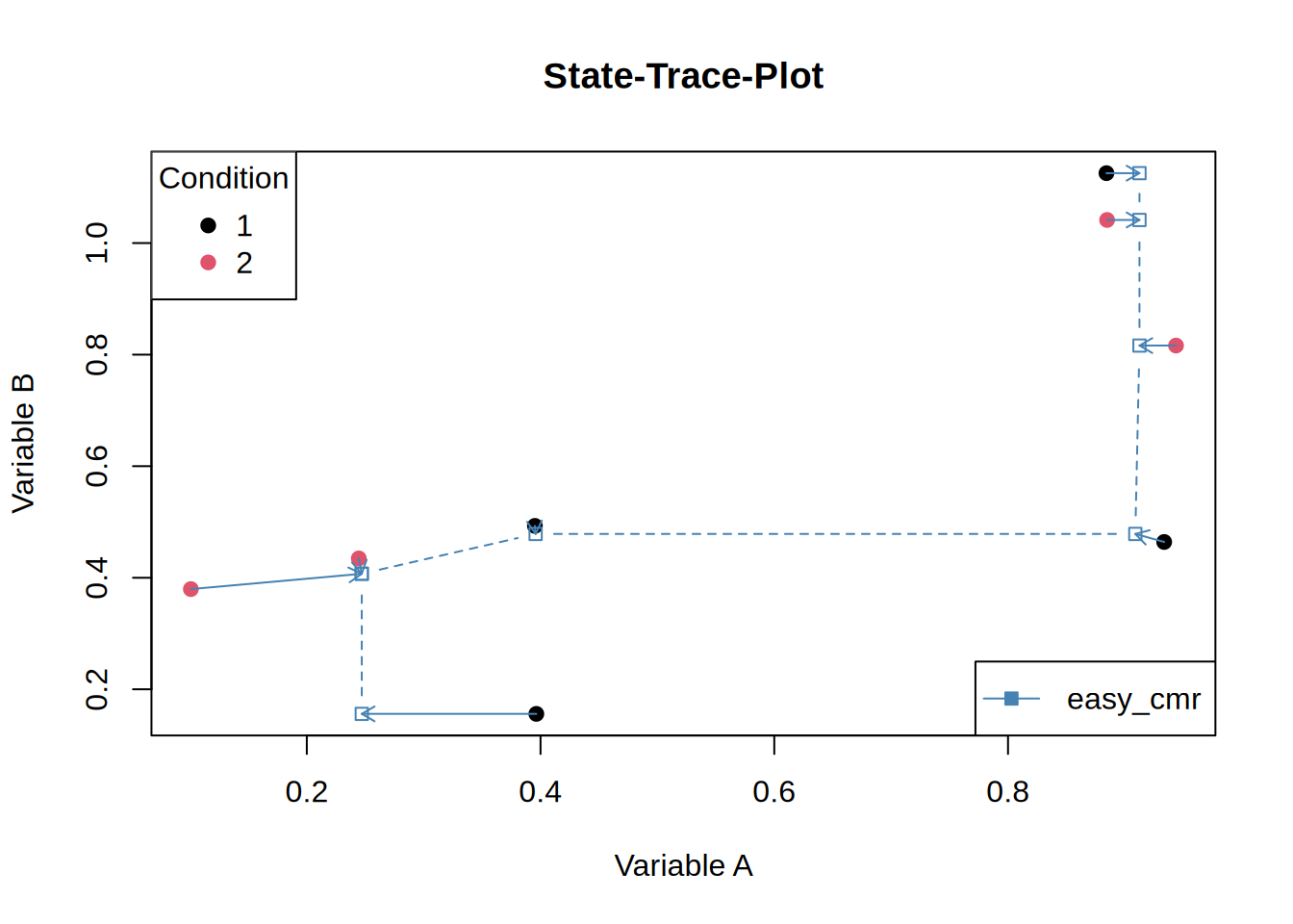
Let’s add some arrows to see which points move:

st_plot(d)
points(res1$X, res1$Y, col = "steelblue", type = "b", pch = 22,
       lty = 2)
arrows(x0 = d_m$X.x, y0 = d_m$Y.x, x1 = d_m$X.y, y1 = d_m$Y.y, col = "steelblue",
       length = 0.08)

legend(
  "bottomright",
  legend = c("easy_cmr"),
  col     = c("steelblue"),
  pch     = c(22),
  lty     = 1,
  pt.bg   = c("steelblue")
)

st_plot(d)
points(res2[order(res2[, 1]), 1], res2[order(res2[,1]), 2], col = "firebrick",
       type = "b", pch = 23, lty = 2)
arrows(x0 = d$X, y0 = d$Y, x1 = res2[, 1], y1 = res2[, 2], col = "firebrick",
       length = 0.08)

legend(
  "bottomright",
  legend = c("jCMRx"),
  col     = c("firebrick"),
  pch     = c(23),
  lty     = 1,
  pt.bg   = c("firebrick")
)

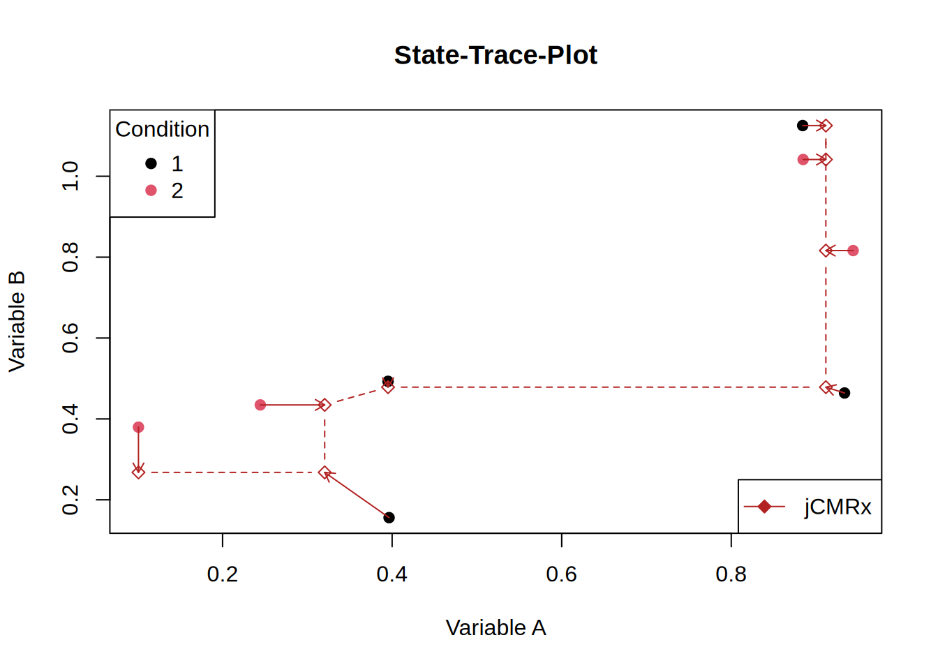
One rather puzzling aspect is that, for jCMRx, the last four points share the same abscissa value, whereas for easy_cmr only the final three points coincide on the abscissa, with the fourth-to-last point shifted slightly further to the left. I am not entirely certain whether this behaviour is expected and whether it is of any substantive relevance.

It is difficult to find an empirical data set that allows for a proper comparison—specifically one that uses the stacmr functions and for which published results are available. In the book by Dunn and Kalish (2018), only a single data set is suitable for a straightforward CMR comparison: the face-inversion data described from page 74 onwards. But even for this data set an algorithm that takes into account the partial order is required.

References

Dunn, John C., and Michael L. Kalish. 2018. State-Trace Analysis. Computational Approaches to Cognition and Perception. Cham: Springer International Publishing. https://doi.org/10.1007/978-3-319-73129-2.