Using Coupled monotonic regression (CMR) in R for State-Trace-Analysis (STA)

The data

We will use the delay data set previously described at https://johannestitz.com/post/2025-10-01-sta-weighting/.

Before we begin, we install all required libraries (using librarian for convenience):

librarian::shelf(monotonicity/stacmr, dplyr, tidyr, ggplot2, 
                 johannes-titz/pirst)

Let us look at the data first:

data(delay)
head(delay)

  participant    delay               structure block     pc
1           1    delay              rule-based    B1 0.3375
2           2 no delay information-integration    B1 0.2875
3           3 no delay              rule-based    B1 0.5250
4           4    delay information-integration    B1 0.3500
5           5    delay              rule-based    B1 0.2375
6           6 no delay information-integration    B1 0.2125

Although this is a mixed design, we can safely ignore the between-subject factor for the present purpose. Let us begin by plotting the data to obtain an initial impression of the patterns:

stats <- sta_stats(
  data = delay,
  col_value = "pc",
  col_participant = "participant",
  col_dv = "structure",
  col_within = "block"
)

means_df1 <- delay %>%
  group_by(structure, block) %>%
  summarize(m = mean(pc))

wide <- tidyr::pivot_wider(means_df1, names_from = structure,
                           values_from = c(m))
p1 <- ggplot(wide, aes(`rule-based`, `information-integration`,
                 color = block, group = block, label = block)) +
  geom_point() +
  geom_text(vjust = 2) +
  theme_classic()
p1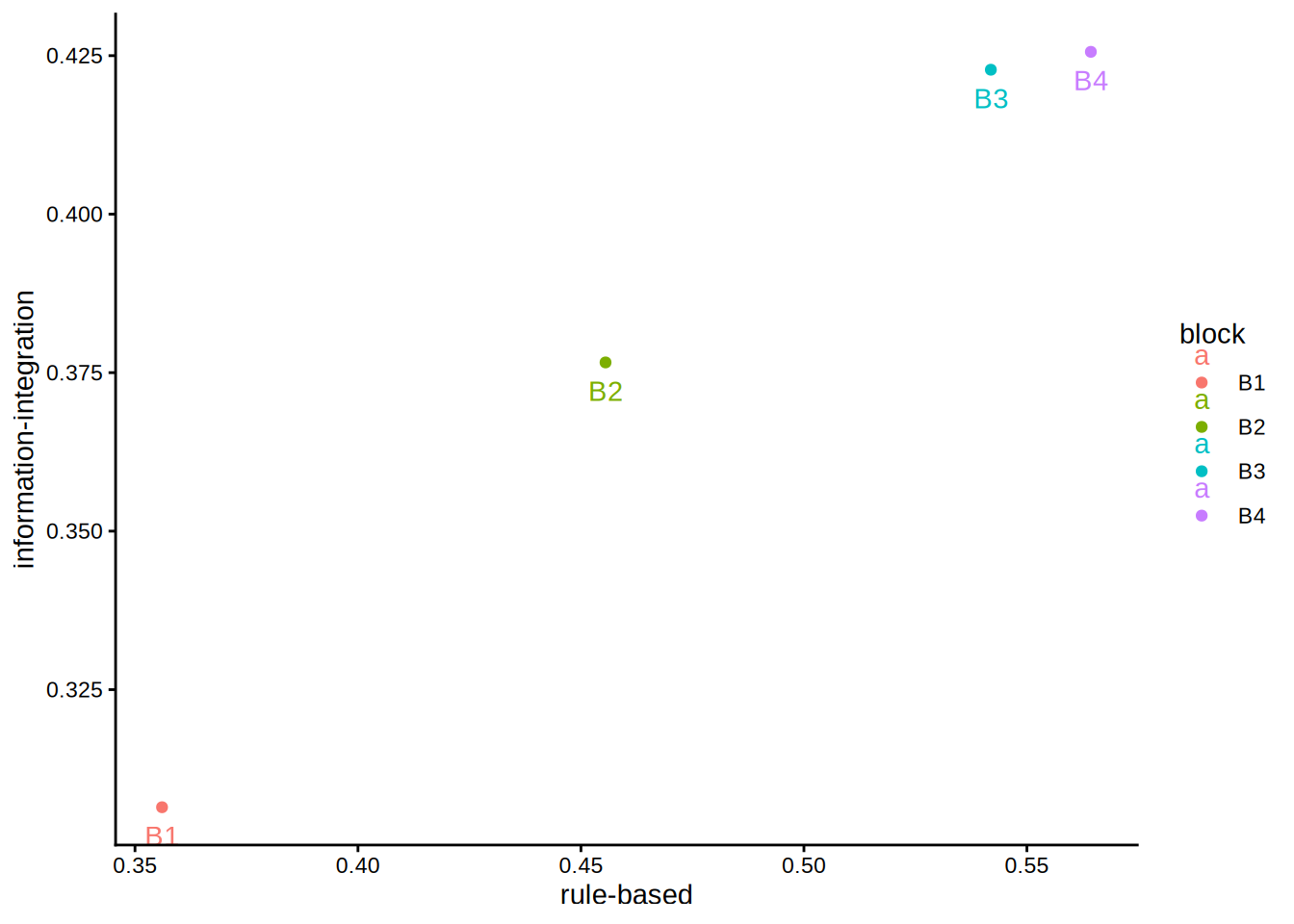

We can already see that the pattern is isotonic, but let us call cmr (from stacmr) nonetheless.

Calling cmr

st_d1 <- cmr(
  data = delay,
  col_value = "pc",
  col_participant = "participant",
  col_dv = "structure",
  col_within = "block",
  nsample = 1e4,
  test = F
)
st_d1

CMR fit to 4 data points with call:
cmr(data = delay, col_value = "pc", col_participant = "participant", 
    col_dv = "structure", col_within = "block", test = F, nsample = 10000)

DVs: rule-based & information-integration 
Within: block 
Between: NA 

Fit value (SSE): 0
Fit difference to MR model (SSE): NA
p-value (based on 0 samples): NA 

summary(st_d1)

CMR fit to 4 data points with call:
cmr(data = delay, col_value = "pc", col_participant = "participant", 
    col_dv = "structure", col_within = "block", test = F, nsample = 10000)

Fit value (SSE): 0
Fit difference to MR model (SSE): NA
p-value (based on 0 samples): NA 

Estimated cell means:
  rule.based information.integration within between
1     0.3561                  0.3065     B1       1
2     0.4555                  0.3766     B2       1
3     0.5419                  0.4228     B3       1
4     0.5643                  0.4256     B4       1

Indeed, we obtain a perfect fit. Note that the between-subject factor was ignored. While the aggregated means are clearly monotonic, we are more interested in each individual participant’s state–trace. However, the cmr function does not operate on individual-level data in this way.

Let us begin by creating a minimal example data set:

delay1 <- delay[as.numeric(delay$participant) <= 2, ]
delay1

    participant    delay               structure block     pc
1             1    delay              rule-based    B1 0.3375
2             2 no delay information-integration    B1 0.2875
131           1    delay              rule-based    B2 0.8875
132           2 no delay information-integration    B2 0.4750
261           1    delay              rule-based    B3 0.9375
262           2 no delay information-integration    B3 0.7000
391           1    delay              rule-based    B4 1.0000
392           2 no delay information-integration    B4 0.7625

We take the first two participants, yielding two dependent variables. Now we call cmr:

st_d1 <- cmr(
  data = delay1,
  col_value = "pc",
  col_participant = "participant",
  col_dv = "structure",
  col_within = "block",
  nsample = 1e4
)
summary(st_d1)

CMR fit to 1 data points with call:
cmr(data = delay1, col_value = "pc", col_participant = "participant", 
    col_dv = "structure", col_within = "block", nsample = 10000)

Fit value (SSE): 0
Fit difference to MR model (SSE): 0
p-value (based on 10000 samples): 1 

Estimated cell means:
  rule.based information.integration between N_rule.based
1     0.7906                  0.5562       1            4

This produces a somewhat unexpected output: there should still be four within-subject blocks, but they have been summarized.

Using data from four participants, we obtain:

delay1 <- delay[as.numeric(delay$participant) <= 4, ]
st_d1 <- cmr(
  data = delay1,
  col_value = "pc",
  col_participant = "participant",
  col_dv = "structure",
  col_within = "block",
  nsample = 1e4
)
summary(st_d1)

CMR fit to 4 data points with call:
cmr(data = delay1, col_value = "pc", col_participant = "participant", 
    col_dv = "structure", col_within = "block", nsample = 10000)

Fit value (SSE): 0.06897
Fit difference to MR model (SSE): 0.06897
p-value (based on 10000 samples): 0 

Estimated cell means:
  rule.based information.integration within between
1     0.4313                  0.3187     B1       1
2     0.7437                  0.3875     B2       1
3     0.9187                  0.6332     B3       1
4     0.9625                  0.6332     B4       1

This looks fine. What happens if we assign a single participant number?

delay1$participant <- 1
st_d1 <- cmr(
  data = delay1,
  col_value = "pc",
  col_participant = "participant",
  col_dv = "structure",
  col_within = "block",
  nsample = 1e4
)
summary(st_d1)

CMR fit to 1 data points with call:
cmr(data = delay1, col_value = "pc", col_participant = "participant", 
    col_dv = "structure", col_within = "block", nsample = 10000)

Fit value (SSE): 0
Fit difference to MR model (SSE): 0
p-value (based on 10000 samples): 1 

Estimated cell means:
  rule.based information.integration between N_rule.based
1     0.7906                  0.5562       1            4

The data are aggregated once again, indicating that the current interface is not suitable for analyzing individual-level data. We could explore the lower-level functions that handle data preparation, or we could examine the wrappers that directly call the Java problem and solver functions.

Calling jCMRx

The structure and functions of the stacmr package are not well documented, and the Java wrappers add complexity. However, the most relevant component for default data appears to be jCMRx.R (the meaning of x is unclear), which serves as a wrapper for the CMRxProblemMaker and ParCMRxSolver Java functions. Let us take a closer look:

jCMRx <- function(d, model, E) {
  nVar <- length(d)
  nCond <- length(d[[1]]$means)
  
  if (missing("model")) { 
    model <- matrix(1, nVar, 1)
  }

  problemMaker <- new(J("au.edu.adelaide.fxmr.model.CMRxProblemMaker"))
  
  .jcall(problemMaker,returnSig = "V","setModel",.jarray(model, dispatch = T))
  for (i in 1:nVar){
    .jcall(problemMaker,returnSig = "V","addMeanArray",.jarray(d[[i]]$means, dispatch = T))
    .jcall(problemMaker,returnSig = "V","addWeightArray",.jarray(d[[i]]$weights, dispatch = T))
  }

  if (!missing("E") && length(E) > 0) {
    if (is.list(E) && is.list(E[[1]])){
      #3d list, different constrains for each variable
      nE <- length(E)
      for(iVar in 1:nVar){
        Ecur <- E[[iVar]]
        index <- problemMaker$initAdj()
        if (length(Ecur) > 0){
          for (j in 1:length(Ecur)){
            problemMaker$addAdj(nCond, index, as.integer(Ecur[[j]]))
          }
        }
      }
    }else if (is.list(E)){
      #Same list for all variables
      index = problemMaker$initAdj();
      for (j in 1:length(E)){
        problemMaker$addAdj(nCond, index, as.integer(E[[j]]));
      }
      problemMaker$dupeAdj(nVar);
    }
  }
  
  cmrxSolver <- new(J("au.edu.adelaide.fxmr.model.ParCMRxSolver"))
  problem <- problemMaker$getProblem()
  solution <- cmrxSolver$solve(problem)
  fVal <- .jcall(solution,"getFStar",returnSig = "D")
  xMatrix <- t(.jcall(solution,"getXStar",returnSig = "[[D",evalArray=TRUE,simplify = TRUE))
  
  return(list(fval=fVal, x=xMatrix))
}

Actually, not much is happening at this stage. Although d contains various components, only the means and weights are passed to the Java functions. Additionally, the model is required, along with the partial order E, which is indeed optional. I am not entirely sure what model represents, but if omitted, it is automatically set to a vector of 1s with length equal to the number of dependent variables.

The intermediate section involving the adjacency matrix primarily handles the partial order E, which is not our focus here. Therefore, creating a custom call to the Java functions should be relatively straightforward. We can test this approach with a minimal example as a proof of concept.

First, let us create some basic data and run Lukas’ simplified version of cmr:

set.seed(1)
dsim <- pirstsim(cases = 1, nmeasures = 1, noise = .1)
res_easy_cmr <- pirst:::easy_cmr(dsim)

We can now invoke the jCMRx function from the Java library:

d <- vector("list", 2)
d[[1]]$means <- dsim$X
d[[2]]$means <- dsim$Y
d[[1]]$weights <- diag(nrow = length(dsim$X))
d[[2]]$weights <- diag(nrow = length(dsim$Y))
res <- stacmr:::jCMRx(d)
res_jCMRx <- res$x[order(res$x[, 1]), ]

Note that jCMRx expects a list containing two lists: one for means and one for weights. As mentioned earlier, this represents the minimum required input. Also, the weights must be provided as a matrix. Here, we simply set all weights to 1, assuming independence (diagonal matrix with 1s ).

The difference between the results is negligible, likely attributable to rounding errors.

as.matrix(res_easy_cmr[, 1:2]) - res_jCMRx

              X Y
1  4.752868e-07 0
5  4.560145e-07 0
6 -9.313013e-07 0
2  0.000000e+00 0
3  0.000000e+00 0
7  0.000000e+00 0
4  0.000000e+00 0
8  0.000000e+00 0

Thus, we now have a relatively straightforward method to run a coupled monotonic regression on arbitrary data in R, including single-participant datasets. This capability is crucial for our work.

The next steps will involve testing whether Lukas’ cmr implementation handles more complex scenarios with larger datasets and more violations of monotonicity. Benchmarking will also be important: while cmr is probably not a bottleneck for PIRST, if the Java libraries are significantly faster, it may be worth either optimizing Lukas’ simple version for speed or implementing a C++ version. The core algorithm itself is relatively concise. Another important step will be to incorporate correct weighting for different experimental designs.

References

Benjamin, Aaron S., Michael L. Griffin, and Jeffrey A. Douglas. 2019. “A Nonparametric Technique for Analysis of State-Trace Functions.” Journal of Mathematical Psychology 90 (June): 88–99. https://doi.org/10/gn2mk8.
Dunn, John C., and Michael L. Kalish. 2018. State-Trace Analysis. Computational Approaches to Cognition and Perception. Cham: Springer International Publishing. https://doi.org/10.1007/978-3-319-73129-2.