  participant    delay               structure block     pc
1           1    delay              rule-based    B1 0.3375
2           2 no delay information-integration    B1 0.2875
3           3 no delay              rule-based    B1 0.5250
4           4    delay information-integration    B1 0.3500
5           5    delay              rule-based    B1 0.2375
6 6 no delay information-integration B1 0.2125Weighting in Within-Subject-Design State-Trace Analysis (STA)
R
statistics
STA
Recently, I revisited the concept of STA to deepen my understanding and examined an example from Dunn and Kalish (2018). The example is based on a memory experiment reported in Dunn, Newell, and Kalish (2012), which used one between-subjects variable (feedback delay vs. no delay) and one within-subjects variable (training block, 1–4). The two dependent variables were proportion correct for rule-based (RB) and information-integration (II) category-learning tasks.
RB tasks are tasks for which a simple, verbalizable rule can be devised (e.g., “If the value x is greater than c, then it belongs to category A”). II tasks, by contrast, depend on implicit learning processes because no easily verbalizable rule exists. In the experiment, 500 ms (no-delay condition) or 5000 ms (delay condition) after stimulus presentation, a Gabor patch mask was shown.
As far as I understand, the underlying idea is that, for RB learning, feedback delay is not particularly detrimental because learners can hold candidate rules in working memory and evaluate feedback later. In contrast, II learning relies on forming stimulus–response associations through procedural learning mechanisms, which require temporal contiguity between response and feedback. Delayed feedback therefore disrupts II learning more strongly.
Note that in the paper only participants with an accuracy of at least 27% were included, whereas in the book all participants are analyzed.
We now load the required libraries and the dataset. Package management is handled via librarian.
Let us first inspect the data visually by drawing a plot:
stats <- sta_stats(
  data = delay,
  col_value = "pc",
  col_participant = "participant",
  col_dv = "structure",
  col_within = "block",
  col_between = "delay"
)

means_df1 <- delay %>%
  group_by(structure, delay, block) %>%
  summarize(m = mean(pc))

wide <- tidyr::pivot_wider(means_df1, names_from = structure,
                           values_from = c(m))
p1 <- ggplot(wide, aes(`rule-based`, `information-integration`,
                 color = delay, group = delay, label = block)) +
  geom_point() +
  geom_text(vjust = 2) +
  theme_classic()
p1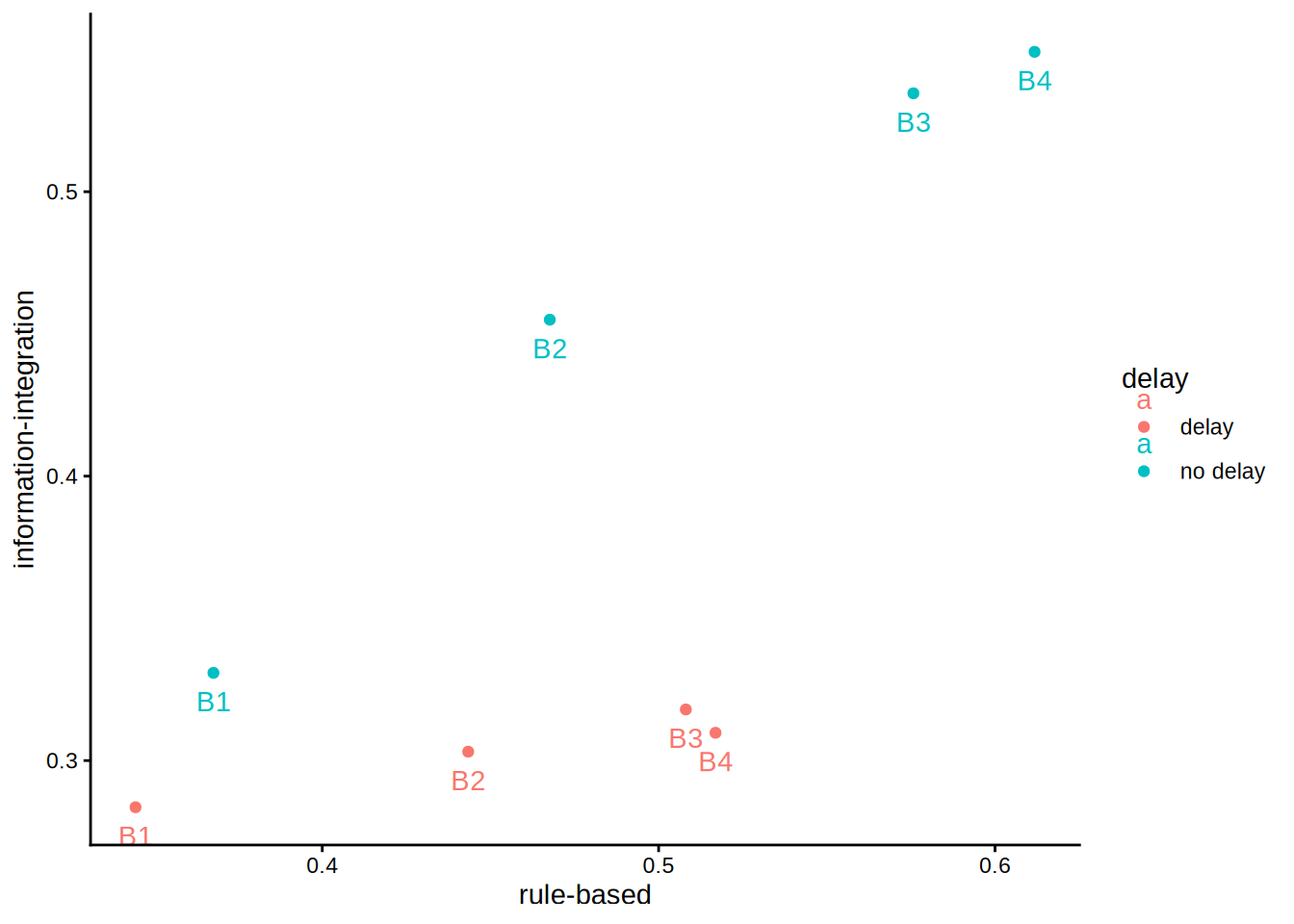
An initial inspection reveals a violation of monotonicity, though this will not be the main focus today. First, we want to fit a partial-order model. Two constraints are relevant. First, within each block the delay group should perform worse than the no-delay group; this constraint is already satisfied and requires no data adjustment. Second, performance should increase monotonically from block 1 to block 4; this holds except for the delay condition in block 3 versus block 4. The partial-order model corrects for this discrepancy because the non-monotonic pattern is theoretically implausible and should be attributed to measurement or other error. In stacmr we apply mr (monotonic regression) and plot the optimal solution.
Note that for the delay data the order of factor-levels corresponds to the expected partial order. Therefore, partial = "auto" can be used to enforce this order.
mr_d1 <- mr(
  data = delay,
  col_value = "pc",
  col_participant = "participant",
  col_dv = "structure",
  col_within = "block",
  col_between = "delay",
  nsample = 10,
  partial = "auto"
)

mr_d1_s <- summary(mr_d1)
MR fit to 8 data points with call:
mr(data = delay, col_value = "pc", col_participant = "participant",
    col_dv = "structure", col_within = "block", col_between = "delay",
    partial = "auto", nsample = 10)

Fit value (SSE): 0.1721
p-value (based on 10 samples): 0.7

Estimated cell means:
  rule.based information.integration within  between
1     0.3445                  0.2830     B1    delay
2     0.4434                  0.3034     B2    delay
3     0.5081                  0.3149     B3    delay
4     0.5169                  0.3149     B4    delay
5     0.3676                  0.3308     B1 no delay
6     0.4676                  0.4550     B2 no delay
7     0.5757                  0.5346     B3 no delay
8     0.6118                  0.5492     B4 no delay
wide <- cbind(wide, mr_d1_s)
p1 + geom_line(data = wide, aes(rule.based, information.integration))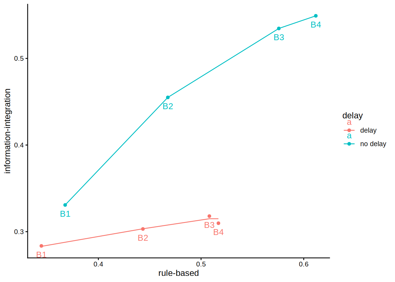
Indeed, this resolves the B3/B4 non-monotonicity for II. Interestingly, however, the model also slightly adjusts the position of all other means:
             rule.based1              rule.based2              rule.based3
            0.000000e+00             0.000000e+00             0.000000e+00
             rule.based4              rule.based5              rule.based6
            0.000000e+00             0.000000e+00             0.000000e+00
             rule.based7              rule.based8 information.integration1
            0.000000e+00             0.000000e+00             5.496299e-04
information.integration2 information.integration3 information.integration4
           -2.359129e-04             3.045620e-03            -5.157505e-03
information.integration5 information.integration6 information.integration7
           -1.398881e-14            -1.088019e-14            -8.659740e-15
information.integration8
           -1.487699e-14
In Dunn and Kalish (2018), the lowest value of the monotonic regression (MR) model for the delay condition is 0.2830, whereas the original observed value was 0.2836. Why does this point shift at all? The reason lies in the within-subject structure of the experiment, which requires a different weighting procedure: the values for B1 through B4 are correlated. Higher scores in B1 tend to co-occur with higher scores in B2, B3, and B4. Consequently, when one point violates the monotonicity constraint, the optimal solution typically involves adjusting several points simultaneously—even if only minimally. This interdependence explains the small shifts.
How, then, is the weighting implemented in this particular case?
Correct weighting
The general formula is:
\[W = N_X S_X^{-1}\]
The corresponding weights can, in fact, be inspected in stacmr via:
V <- stats$rule.based$weights
W <- stats$information.integration$weights
V
[,1] [,2] [,3] [,4] [,5] [,6]
[1,] 3192.7243 -1210.688 436.2617 -356.4355 0.00000 0.0000
[2,] -1210.6877 3460.623 -1937.4585 -669.5800 0.00000 0.0000
[3,] 436.2617 -1937.459 4287.8355 -2319.4907 0.00000 0.0000
[4,] -356.4355 -669.580 -2319.4907 3033.3542 0.00000 0.0000
[5,] 0.0000 0.000 0.0000 0.0000 4909.21477 -2498.4605
[6,] 0.0000 0.000 0.0000 0.0000 -2498.46049 3232.6705
[7,] 0.0000 0.000 0.0000 0.0000 287.22054 -1204.0883
[8,] 0.0000 0.000 0.0000 0.0000 -74.88846 -379.6758
[,7] [,8]
[1,] 0.0000 0.00000
[2,] 0.0000 0.00000
[3,] 0.0000 0.00000
[4,] 0.0000 0.00000
[5,] 287.2205 -74.88846
[6,] -1204.0883 -379.67584
[7,] 2727.5721 -1349.75598
[8,] -1349.7560 1780.38691W [,1] [,2] [,3] [,4] [,5] [,6]
[1,] 6023.1736 -954.9243 -777.7281 226.2976 0.0000 0.00000
[2,] -954.9243 4904.9758 -1456.5032 -1186.2243 0.0000 0.00000
[3,] -777.7281 -1456.5032 4180.2981 -1616.1973 0.0000 0.00000
[4,] 226.2976 -1186.2243 -1616.1973 3192.4727 0.0000 0.00000
[5,] 0.0000 0.0000 0.0000 0.0000 5917.7959 -2643.97092
[6,] 0.0000 0.0000 0.0000 0.0000 -2643.9709 3345.70934
[7,] 0.0000 0.0000 0.0000 0.0000 -307.5252 -1229.73039
[8,] 0.0000 0.0000 0.0000 0.0000 -204.0576 -12.65251
[,7] [,8]
[1,] 0.0000 0.00000
[2,] 0.0000 0.00000
[3,] 0.0000 0.00000
[4,] 0.0000 0.00000
[5,] -307.5252 -204.05759
[6,] -1229.7304 -12.65251
[7,] 4018.6958 -2498.85536
[8,] -2498.8554 2771.05065Now, we are able to reproduce the correct fit value:
     [,1]
[1,] 0 [,1]
[1,] 0.1721286The last two values are added, but since the first is zero, the final value corresponds to the MR model’s fitted estimate:
mr_d1$fit[1] 0.1721286If we compare this with a naïve approach—using only the inverse of the variance of the means as weights—we obtain a poorer fit once the correct weighting is applied in the final fit calculation:
          [,1]
[1,] 0.1757721
Thus, the weighting procedure matters and explains why points that already satisfy monotonicity may still shift. Because the values are interdependent, adjustments to one point can propagate to others, even if they initially appear perfectly positioned.
Some more background
I tried to teach myself linear algebra, but I only covered the basics without much focus on statistical applications, so I don’t fully understand all the details yet. But the basic idea is that the sampling variance of a linear combination is given by:
\[\text{Var}(c^T X) = c^T \Sigma c,\]
where \(c\) is the contrast vector and \(\Sigma\) the covariance matrix. When you check this formula using a simple t-test example, it actually works out as expected.
Means vector:
\[ \bar{\mathbf X} = \begin{bmatrix} \bar X_A\\[4pt] \bar X_B \end{bmatrix} = \begin{bmatrix} 10\\[4pt] 12 \end{bmatrix}. \] Covariance:
\[ \Sigma = \begin{bmatrix} \mathrm{Var}(\bar X_A) & \mathrm{Cov}(\bar X_A,\bar X_B)\\[6pt] \mathrm{Cov}(\bar X_B,\bar X_A) & \mathrm{Var}(\bar X_B) \end{bmatrix} = \begin{bmatrix} 0.1333 & 0.1667\\[6pt] 0.1667 & 0.3000 \end{bmatrix}. \]
Contrast vector:
\[ \mathbf c = \begin{bmatrix} 1\\[4pt] -1 \end{bmatrix}. \]
Mean Difference:
\[ \hat D = \mathbf c^\top \bar{\mathbf X} = \begin{bmatrix} 1 & -1 \end{bmatrix} \begin{bmatrix} 10\\[4pt] 12 \end{bmatrix} = -2. \] Variance of Mean Difference:
\[ \mathrm{Var}(\hat D) = \mathbf c^\top \Sigma \mathbf c = \begin{bmatrix} 1 & -1 \end{bmatrix} \begin{bmatrix} 0.1333 & 0.1667\\[4pt] 0.1667 & 0.3000 \end{bmatrix} \begin{bmatrix} 1\\[4pt] -1 \end{bmatrix}. \]
\[ \Sigma \mathbf c = \begin{bmatrix} 0.1333 - 0.1667\\[4pt] 0.1667 - 0.3000 \end{bmatrix} = \begin{bmatrix} -0.0334\\[4pt] -0.1333 \end{bmatrix}, \qquad \mathbf c^\top (\Sigma \mathbf c) = -0.0334 + 0.1333 = 0.10. \]
\[ \mathrm{SE}(\hat D) = \sqrt{\mathbf c^\top \Sigma \mathbf c} = \sqrt{0.10} = 0.316. \] t-value:
\[ t = \frac{\mathbf c^\top \bar{\mathbf X} - 0}{\sqrt{\mathbf c^\top \Sigma \mathbf c}} = \frac{-2}{0.316} = -6.33. \]
The interesting feature of the weight matrix is its general applicability. In a purely between-subjects design, the weight matrix will have nonzero entries only along the diagonal. While covariances may not always be exactly zero, the pairwise sample sizes for between-subject comparisons are zero, so off-diagonal weights do not contribute. In a within-subjects design, both the covariance matrix and the sample-size matrix typically contain nonzero entries throughout. In mixed designs, some covariances are zero while others are not. This flexibility makes the weight matrix a powerful tool for a wide range of experimental designs.
References
Dunn, John C., and Michael L. Kalish. 2018. State-Trace Analysis. Computational Approaches to Cognition and Perception. Cham: Springer International Publishing. https://doi.org/10.1007/978-3-319-73129-2.
Dunn, John C., Ben R. Newell, and Michael L. Kalish. 2012. “The Effect of Feedback Delay and Feedback Type on Perceptual Category Learning: The Limits of Multiple Systems.” Journal of Experimental Psychology: Learning, Memory, and Cognition 38 (4): 840–59. https://doi.org/10.1037/a0027867.